Introduction to ppforest2
introduction.Rmdppforest2 builds oblique decision trees and random forests using projection pursuit. Instead of splitting on a single variable at each node, it finds a linear combination of variables that best separates the groups.
Single tree
Train a projection-pursuit tree on the iris dataset:
library(ppforest2)

tree <- pptr(Species ~ ., data = iris, seed = 0)
tree
#>
#> Call: pptr(formula = Species ~ ., data = iris, seed = 0)
#>
#> Projection-Pursuit Oblique Decision Tree:
#> If ([ 0 -0.04 0.03 0.03 ] * x) < 0.01580044:
#>   Predict: setosa
#> Else:
#>  If ([ 0 0.03 -0.06 -0.15 ] * x) < -0.4503323:
#>    Predict: virginica
#>  Else:
#>    Predict: versicolor
The tree splits on linear projections of the features. Use
summary() to see variable importance:
summary(tree)
#>
#> Projection-Pursuit Oblique Decision Tree
#>
#> pp method: PDA (lambda=0.5)
#> vars method: All variables
#> cutpoint method: Mean of means
#> stop rule: Pure node
#> binarize method: Largest gap
#> grouping method: By label
#> leaf method: Majority vote
#>
#>
#> Data Summary:
#>   observations: 150
#>   features:     4
#>   groups:       3
#>   group names:  setosa, versicolor, virginica
#>   formula:      Species ~ Sepal.Length + Sepal.Width + Petal.Length + Petal.Width -      1
#>
#> Confusion Matrix:
#>
#>             Predicted
#> Actual       setosa versicolor virginica
#>   setosa         50          0         0
#>   versicolor      0         47         3
#>   virginica       0          3        47
#>
#> Training error: 4%
#>
#> Variable Importance:
#>
#>       Variable         σ  Projection
#> 1  Petal.Width 0.7622377 0.067165621
#> 2 Petal.Length 1.7652982 0.064908713
#> 3  Sepal.Width 0.4358663 0.011343628
#> 4 Sepal.Length 0.8280661 0.001772132
#>
#> Note: Variable importance was calculated using scaled coefficients (|a_j| * σ_j).
#> Variable contributions can only be theoretically interpreted as such
#> if the model was trained on scaled data. Scaling also changes the
#> projection-pursuit optimization, which may affect the resulting tree.
Predict new observations:
Random forest
Train a forest of 100 trees, each considering 2 randomly chosen variables at each split:
forest <- pprf(Species ~ ., data = iris, size = 100, n_vars = 2, seed = 0)
summary(forest)
#>
#> Random Forest of Projection-Pursuit Oblique Decision Trees
#>
#> Size: 100 trees
#> pp method: PDA (lambda=0.5)
#> vars method: Uniform random (count=2)
#> cutpoint method: Mean of means
#> stop rule: Pure node
#> binarize method: Largest gap
#> grouping method: By label
#> leaf method: Majority vote
#>
#>
#> Data Summary:
#>   observations: 150
#>   features:     4
#>   groups:       3
#>   group names:  setosa, versicolor, virginica
#>   formula:      Species ~ Sepal.Length + Sepal.Width + Petal.Length + Petal.Width -      1
#>
#> Training Confusion Matrix:
#>
#>             Predicted
#> Actual       setosa versicolor virginica
#>   setosa         50          0         0
#>   versicolor      0         48         2
#>   virginica       0          5        45
#>
#> Training error: 4.67%
#>
#> OOB Confusion Matrix:
#>
#>             Predicted
#> Actual       setosa versicolor virginica
#>   setosa         50          0         0
#>   versicolor      0         48         2
#>   virginica       0          4        46
#>
#> OOB error: 4%
#>
#> Variable Importance:
#>
#>       Variable         σ  Projection    Weighted   Permuted
#> 1 Petal.Length 1.7652982 0.060925536 0.044617556 0.31747234
#> 2  Petal.Width 0.7622377 0.045294985 0.035571091 0.24510610
#> 3 Sepal.Length 0.8280661 0.013997004 0.006649137 0.06048262
#> 4  Sepal.Width 0.4358663 0.007664503 0.005792385 0.03662244
#>
#> Note: Variable importance was calculated using scaled coefficients (|a_j| * σ_j).
#> Variable contributions can only be theoretically interpreted as such
#> if the model was trained on scaled data. Scaling also changes the
#> projection-pursuit optimization, which may affect the resulting tree.
The summary shows the OOB (out-of-bag) error estimate and three variable importance measures:
- Projection: average absolute projection coefficient across all splits
- Weighted: projection importance weighted by the number of observations routed through each node
- Permuted: decrease in OOB accuracy when each variable is permuted
Predict with class probabilities:
probs <- predict(forest, iris[1:5, ], type = "prob")
probs
#>   setosa versicolor virginica
#> 1      1          0         0
#> 2      1          0         0
#> 3      1          0         0
#> 4      1          0         0
#> 5      1          0         0
Visualization
ppforest2 provides several plot types via plot()
(requires ggplot2):
# Tree structure with projected data histograms at each node
plot(tree, type = "structure")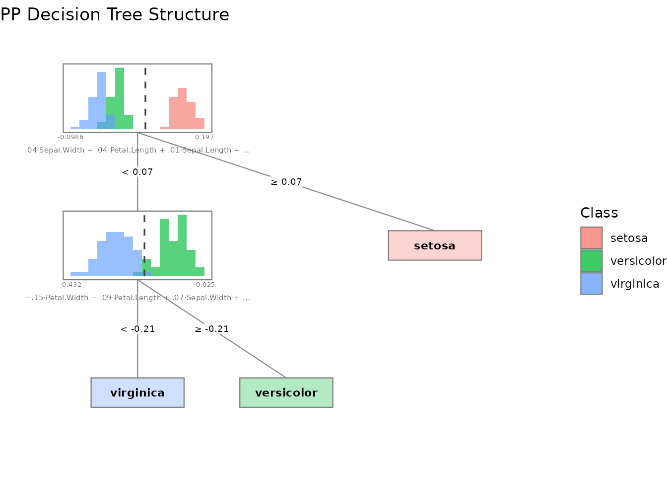
# Variable importance bar chart
plot(tree, type = "importance")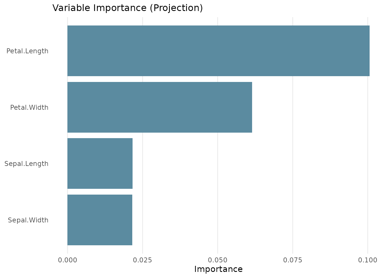
# Data projected onto the first split's projection vector
plot(tree, type = "projection")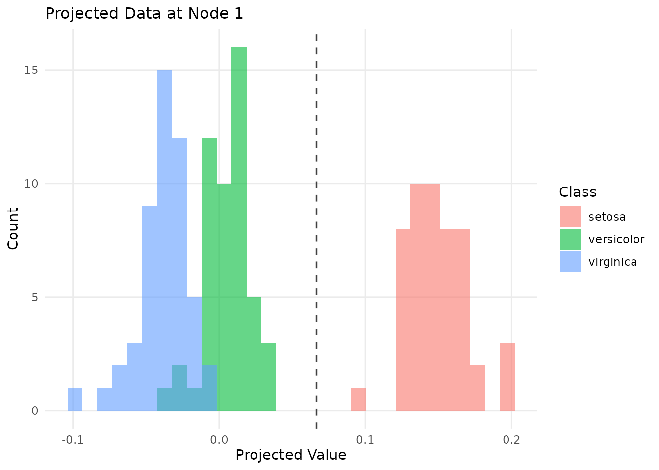
# Decision boundaries for two selected variables
plot(tree, type = "boundaries")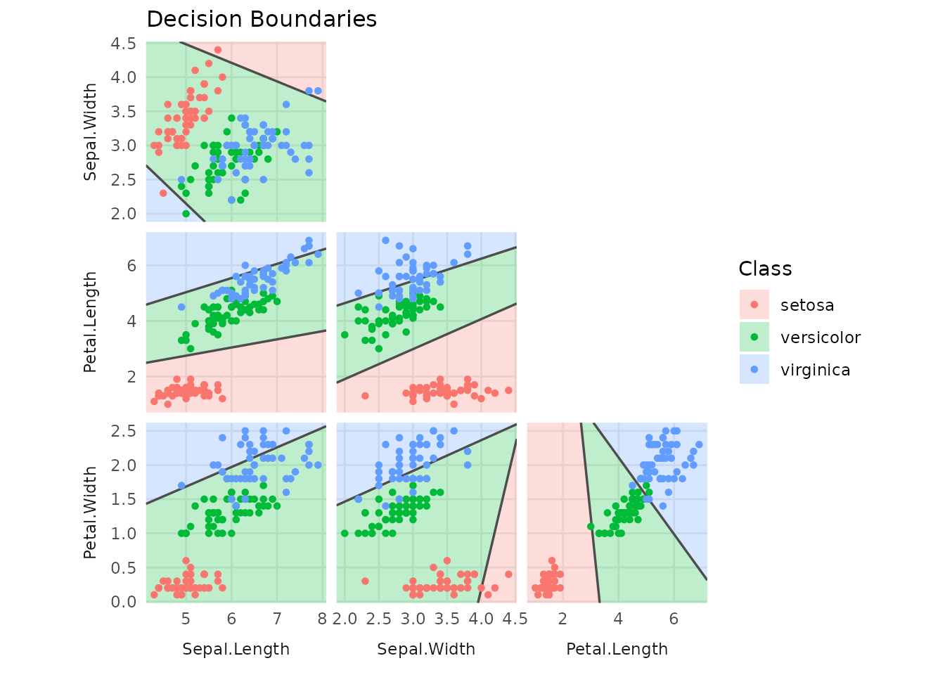
For forests, variable importance is the only global visualization
available. Individual trees can be plotted by specifying a
tree_index.
plot(forest)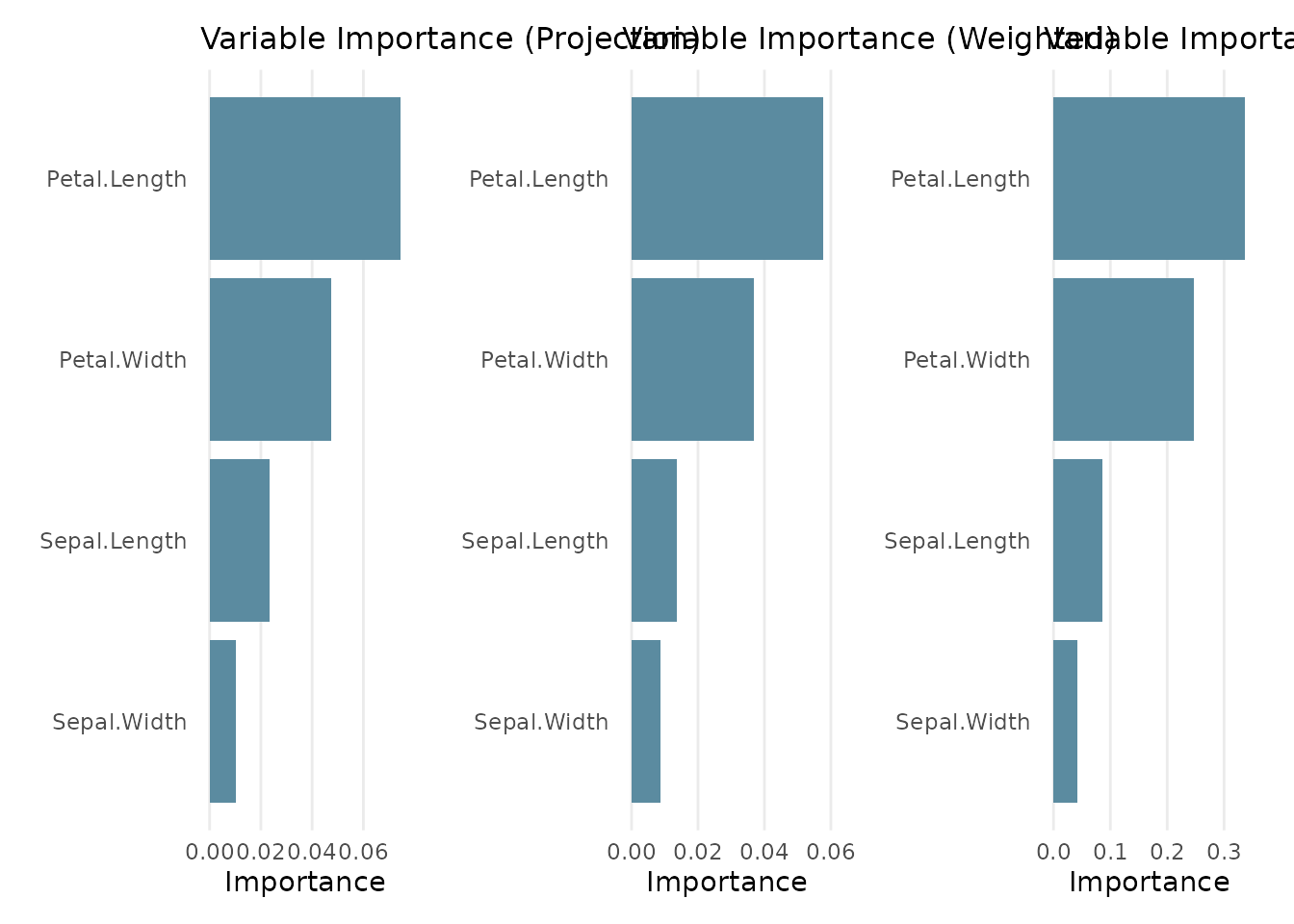
plot(forest, type = "structure", tree_index = 1)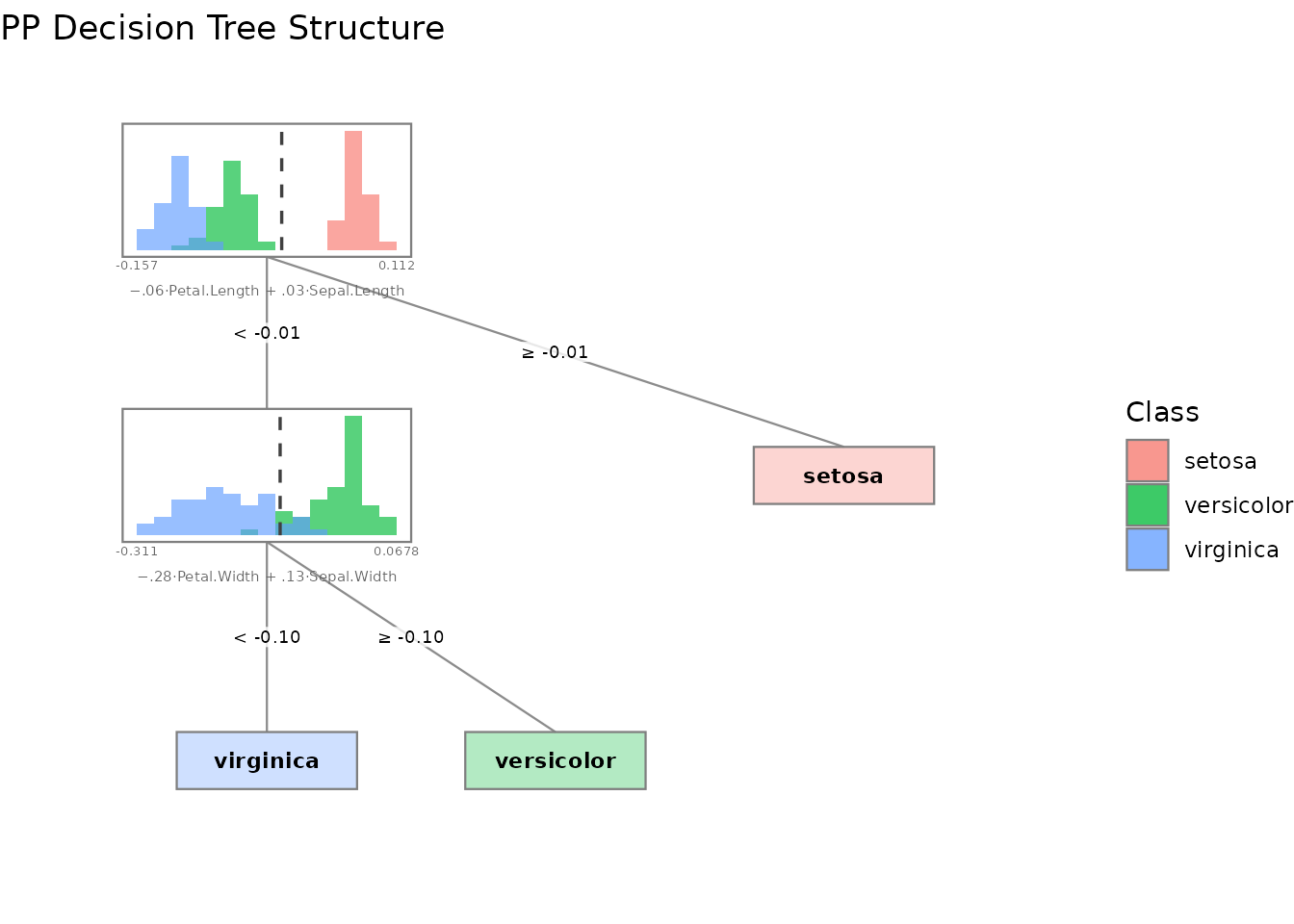
Regularization with PDA
Set lambda > 0 to use Penalized Discriminant Analysis
instead of LDA. This can help when features are highly correlated:
tree_pda <- pptr(Species ~ ., data = iris, lambda = 0.5, seed = 0)
summary(tree_pda)
#>
#> Projection-Pursuit Oblique Decision Tree
#>
#> pp method: PDA (lambda=0.5)
#> vars method: All variables
#> cutpoint method: Mean of means
#> stop rule: Pure node
#> binarize method: Largest gap
#> grouping method: By label
#> leaf method: Majority vote
#>
#>
#> Data Summary:
#>   observations: 150
#>   features:     4
#>   groups:       3
#>   group names:  setosa, versicolor, virginica
#>   formula:      Species ~ Sepal.Length + Sepal.Width + Petal.Length + Petal.Width -      1
#>
#> Confusion Matrix:
#>
#>             Predicted
#> Actual       setosa versicolor virginica
#>   setosa         50          0         0
#>   versicolor      0         47         3
#>   virginica       0          3        47
#>
#> Training error: 4%
#>
#> Variable Importance:
#>
#>       Variable         σ  Projection
#> 1  Petal.Width 0.7622377 0.067165621
#> 2 Petal.Length 1.7652982 0.064908713
#> 3  Sepal.Width 0.4358663 0.011343628
#> 4 Sepal.Length 0.8280661 0.001772132
#>
#> Note: Variable importance was calculated using scaled coefficients (|a_j| * σ_j).
#> Variable contributions can only be theoretically interpreted as such
#> if the model was trained on scaled data. Scaling also changes the
#> projection-pursuit optimization, which may affect the resulting tree.
Explicit strategy selection
For more control, you can pass strategy objects directly instead of
using the shortcut parameters (lambda, n_vars,
p_vars). This is equivalent but makes the strategy choice
explicit:
# These two calls produce identical results:
forest_shortcut <- pprf(Species ~ ., data = iris, size = 10, lambda = 0.5, n_vars = 2, seed = 0)

forest_explicit <- pprf(Species ~ ., data = iris, size = 10, pp = pp_pda(0.5), vars = vars_uniform(n_vars = 2), seed = 0)

all.equal(predict(forest_shortcut, iris), predict(forest_explicit, iris))
#> [1] TRUE
Available strategy constructors:
-
pp_pda(lambda)— PDA projection pursuit (lambda = 0for LDA) -
vars_uniform(n_vars)orvars_uniform(p_vars)— random variable selection -
vars_all()— use all variables (default for single trees) -
cutpoint_mean_of_means()— midpoint split rule (default)
Strategy objects can also be passed as engine arguments in parsnip:
library(parsnip)

spec <- pp_rand_forest(trees = 10) |>
  set_engine("ppforest2", pp = pp_pda(0.5), vars = vars_uniform(n_vars = 2)) |>
  set_mode("classification")

fit <- spec |> fit(Species ~ ., data = iris)
predict(fit, iris[1:5, ])
#> # A tibble: 5 × 1
#>   .pred_class
#>   <fct>
#> 1 setosa
#> 2 setosa
#> 3 setosa
#> 4 setosa
#> 5 setosa
Tidymodels integration
ppforest2 integrates with the tidymodels ecosystem via parsnip:
library(parsnip)

# Single tree
spec <- pp_tree(penalty = 0.5) |>
  set_engine("ppforest2") |>
  set_mode("classification")

fit <- spec |> fit(Species ~ ., data = iris)
predict(fit, iris[1:5, ])
#> # A tibble: 5 × 1
#>   .pred_class
#>   <fct>
#> 1 setosa
#> 2 setosa
#> 3 setosa
#> 4 setosa
#> 5 setosa
# Random forest
spec <- pp_rand_forest(trees = 50, mtry = 2, penalty = 0.5) |>
  set_engine("ppforest2") |>
  set_mode("classification")

fit <- spec |> fit(Species ~ ., data = iris)
predict(fit, iris[1:5, ], type = "prob")
#> # A tibble: 5 × 3
#>   .pred_setosa .pred_versicolor .pred_virginica
#>          <dbl>            <dbl>           <dbl>
#> 1            1                0               0
#> 2            1                0               0
#> 3            1                0               0
#> 4            1                0               0
#> 5            1                0               0